Machine Learning for the Rest of Us

ChatGPT, DALL-E, and Stable Diffusion have renewed the interest of many in Machine Learning, myself included. So, I finally mustered the courage to dive deeper into ML fundamentals and theory.

If you’re like me and are fascinated and distressed by the amount of catchup needed to learn the theory behind ML, this video and blog post are for you.

In the second part, I’m going to take one of these ML examples and take it all the way to a productive app using DevOps practices like data version tracking with dvc, automation, and continuous integration.

Understanding the Terminology

Before diving into the practical aspects, it’s crucial to familiarize yourself with some fundamental terms and concepts:

• Model: A mathematical representation of the real-world process you wish to predict or understand.
• Target (y): the data we want to predict. For example, the house price or if an image shows an animal or a car.
• Inference: Making predictions using a trained model.
• Features (X): Input variables the model uses to make predictions. For instance, these could be pixels or other attributes extracted from images in a computer vision model.
• Prediction: The output or response the model gives based on the input data.
• Epoch: An iteration over the entire dataset during the training process.
• Loss: A measure of how well the model’s predictions align with the actual data. Lower loss indicates a better model.

Traditional ML vs. Neural Networks

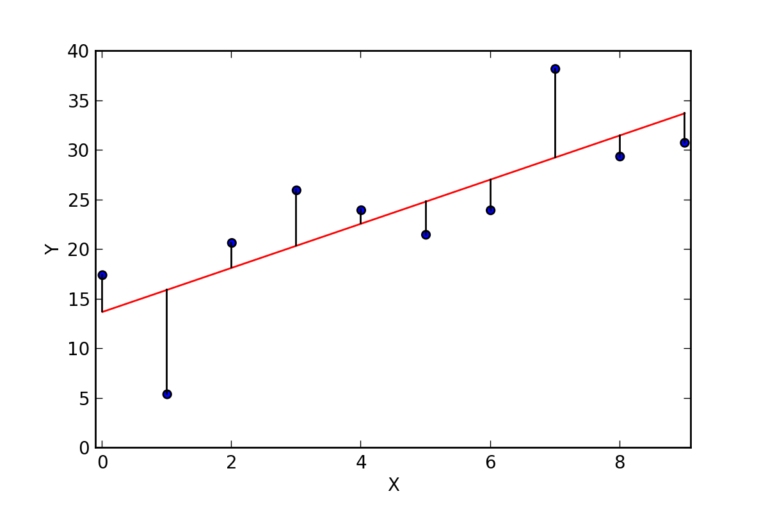
Machine learning can be broadly categorized into traditional and neural network-based approaches. Traditional methods involve well-defined algorithms and steps, like finding a regression function for prediction.

On the other hand, neural networks are used for more complex tasks like image recognition or natural language processing, where the steps for the computer to follow aren’t as clear-cut.

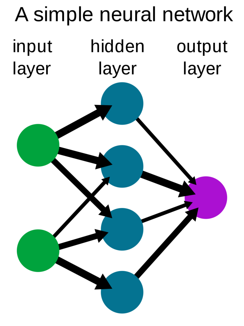
A neural network consists of layers of interconnected neurons. It includes an input layer, several hidden layers where most computations happen, and an output layer that produces the predictions.

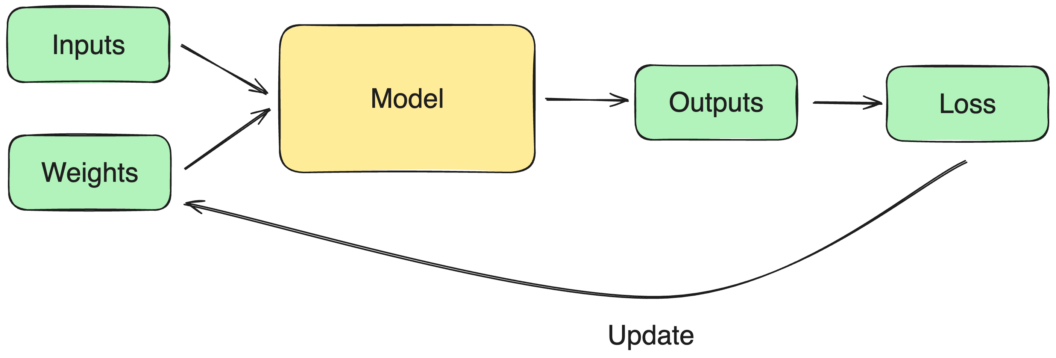
The training process involves:

• Feeding data into the model.
• Calculating the loss (difference between predicted and actual values).
• Adjusting the neurons’ weights iteratively to improve the model’s accuracy.

Getting Started with Kaggle.com

Starting with Kaggle.com is straightforward. You can dive into your first project after creating and verifying your account (which unlocks useful features like internet access in notebooks). The platform allows you to conveniently create notebooks, access GPUs, and add datasets or models.

Example 1: Traditional Machine Learning

Find the notebook here: https://www.kaggle.com/code/tomasfern/optimal-decision-trees/

The first example involves predicting housing prices using traditional machine learning techniques.

Data Preparation

The first step is to load the CSV dataset and remove rows with missing data using dropna(). We tell pandas to delete rows with missing columns with axis=0 and to do it in-place with inplace=True:

import pandas as pd

housing_csv_path = '/kaggle/input/california-housing-prices/housing.csv'
housing = pd.read_csv(housing_csv_path) 

housing.dropna(axis=0, inplace=True)

We can use housing.isna().sum() to verify no rows have missing data. All columns should read 0:

longitude             0
latitude              0
housing_median_age    0
total_rooms           0
total_bedrooms        0
population            0
households            0
median_income         0
median_house_value    0
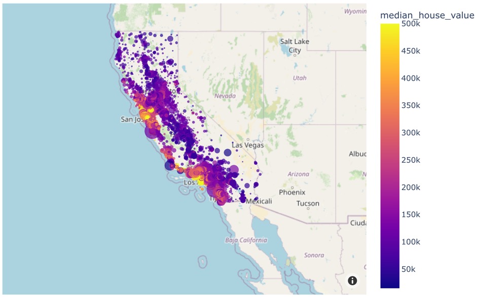
ocean_proximity       0

Next, we can visualize the data by plotting it over a map. The plotly library will help here:

import plotly.express as px

fig = px.scatter_mapbox(housing, lat='latitude', lon='longitude',
                        hover_name='median_house_value',
                        color='median_house_value',
                        size='population',
                        zoom=4, height=600)
fig.update_layout( mapbox_style="open-street-map")
fig.show()

We should get something like this:

Feature Selection

With the data neatly organized, we need to select the features. Remember, these are the columns that we believe have predicting value over the price. Let’s select five features to start. We’ll call these values X:

features = ['longitude', 'latitude', 'households', 'housing_median_age', 'median_income']
X = housing[features]

The value we want to predict is called y and in this case is the median_house_value column:

y = housing['median_house_value']

Let’s call the describe() function to get statistics on both variables. This is X.describe():

count     20433.000000
mean     206864.413155
std      115435.667099
min       14999.000000
25%      119500.000000
50%      179700.000000
75%      264700.000000
max      500001.000000

And this y.describe():

count     20433.000000
mean     206864.413155
std      115435.667099
min       14999.000000
25%      119500.000000
50%      179700.000000
75%      264700.000000
max      500001.000000

Splitting the Data

We’ll split your data into training and validation sets to avoid overfitting (where the model performs well on training data but poorly on unseen data).

We can do this using train_test_split from the SciKit-Learn framework:

from sklearn.model_selection import train_test_split

X_train, X_test, y_train, y_test = train_test_split(X, y, test_size=0.2, random_state=1)

The code takes the features (X), target (y), the number of rows to reserve for validation (0.2 = 20%), and a random state to calculate the split point.

The function returns:

1. X_train: the features for training (without the validation subset)
2. X_test: the features for validation (20% of the original dataset)
3. y_train: the target values for training.
4. y_test: the target values for validation.

Training the Model

We will try a Decision Tree model for our first attempt. To train it, we’ll use the fit() function with the training Features and Targets:

from sklearn.tree import DecisionTreeRegressor

model = DecisionTreeRegressor(random_state=1)
model.fit(X_train, y_train)

After a few seconds, the model should be ready.

Testing the Model

To test the model, we can calculate the difference between the predicted values and the actual target y (the prices in the validation set). We use mean_absolute_error (MAE) for this:

from sklearn.metrics import mean_absolute_error

predictions = model.predict(X_test)
mean_absolute_error(y_test, predictions)

In my example, the MAE for this model is “$43021”. This is our base error. Let’s see if we can improve it.

Finding the Optimal Size

We can control the size of the Decision Tree by changing the max_leaf_nodes. The more leaves, the deeper the model goes. But is a bigger tree better? Not always, there is a point of diminishing returns and then it starts to degrade. This happens because a bigger model can capture spurious data in the dataset. In other words, aberrations are considered valid patterns, leading to worse predictions.

We can find the optimal size by training several models and calculating the error:

def train(max_leaf_nodes, X_train, X_test, y_train, y_test):
    model = DecisionTreeRegressor(max_leaf_nodes=max_leaf_nodes, random_state=1)
    model.fit(X_train, y_train)
    predictions = model.predict(X_test)
    error = mean_absolute_error(y_test, predictions)
    return(error)


for max_leaf_nodes in [5, 50, 500, 5000]:
    error = train(max_leaf_nodes, X_train, X_test, y_train, y_test)
    print("Max leaf nodes: %d  \t ➡ Mean Absolute Error:  %d" %(max_leaf_nodes, error))

The result of this exercise is:

Max Leaf Nodes	Mean Absolute Error
5	$ 63289
50	$ 46528
500	$ 38098
5000	$ 41770

Clearly, the best case happens with 500 nodes.

Random Forests

Random Forests is a collection of decision trees, where each tree differs slightly from the others. We can often produce a better model by averaging or combining the results of different trees.

The code for Random Forest is very similar to the one used in Decision Trees:

from sklearn.ensemble import RandomForestRegressor

model = RandomForestRegressor(random_state=1)
model.fit(X_train, y_train)

Let’s test the error in this model:

from sklearn.metrics import mean_absolute_error

prediction = model.predict(X_test)
mean_absolute_error(y_test, prediction)

As you can see, Random Forest provides better results by default. In this case, I got a MAE of “$31229”. Lower than any other model so far.

Example 2: Neural Network for Computer Vision

Find the notebook here: https://www.kaggle.com/code/tomasfern/cats-or-dogs-classifier

In this exercise, we’re going to fine-tune a Convolutional Neural Network (CNN) to recognize cats and dogs.

Data Preparation

We will use the Oxford-IIIT Pets dataset of over 7000 images of cats and dogs of different breeds.

Cats’ filenames begin with uppercase, while dogs’ begin with lowercase. For this example, we’re going to ignore the breeds altogether.

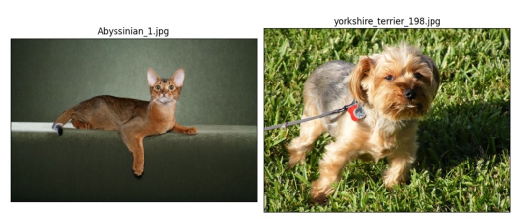
The notebook already has imported the dataset. So, we can access the images directly in the /kaggle mountpoint.

For this example, we’re going to use the FastAI library, a high-level framework that works on top of PyTorch. We define is_cat, which returns True for cats and False for dogs.

Then we create an ImageDataLoader object. This combines the labeling, data splitting (into train and validation subsets), and a resize function.

import numpy as np
from fastai.vision.all import *
path = "/kaggle/input/oxford-iit-pets/images/images/"

# labeling function
def is_cat(x): 
    return x[0].isupper() 

# create data loader "dls"
dls = ImageDataLoaders.from_name_func(
        path, 
        get_image_files(path), 
        valid_pct=0.2, # reserve 20% of images for testing (don't use for training)
        seed=42,       # random split of training/validation sets
        label_func=is_cat, # is_cat is the labeling function (True=Cat, False=Dog)
        item_tfms=Resize(224) # resize data to square 224 px image
)

We can see the labeled images with: dls.valid.show_batch(max_n=8, nrows=2).

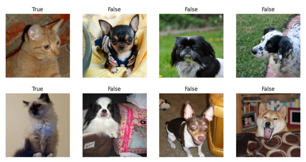
So far, so good.

Fine-tuning a CNN Model

Instead of training a model from scratch, we can use a pre-trained Convolutional Neural Network (CNN). CNNs perform very well for computer vision, so we’ll use ResNet34 as our base model.

Fine-tuning changes the top layer of the model, called the head, to direct it towards responding with True or False for the examples provided. To fine-tune, we can use the vision_learner function in FastAI:

learn = vision_learner(dls, resnet34, metrics=error_rate)
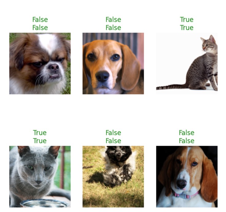
learn.fine_tune(1)

Testing the Model

FastAI runs the validation tests automatically after finishing the fine-tuning. We can see a sample of the results with learn.show_results(max_n=6, figsize=(7,7)).

The confusion matrix shows us how many false positives the testing detected.

interp = ClassificationInterpretation.from_learner(learn)
interp.plot_confusion_matrix()

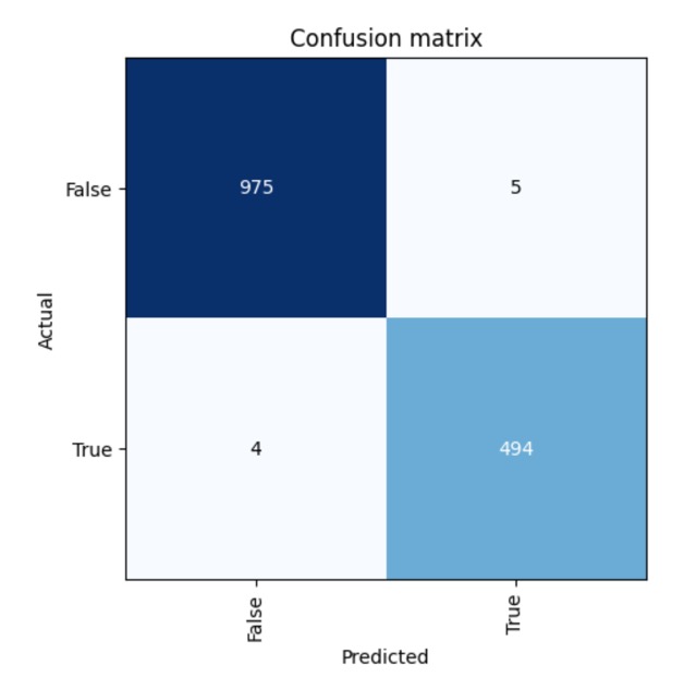
In this case, we had 9 misclassified images. The blue diagonal shows the correct predictions.

To see the top misclassified images, we can use inter.plot_top_losses(5, nrows=1).

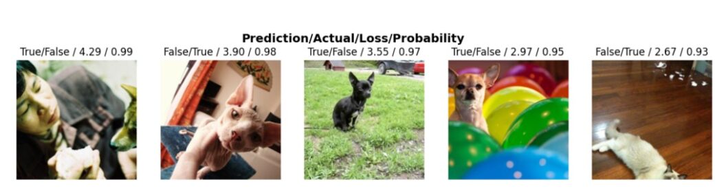
The plot shows misclassified images (cats detected as dogs and the other way around) and inaccurate classifications with low confidence. We can use these examples to see the weaknesses of our model.

Conclusion

Exploring machine learning through practical projects on platforms like Kaggle provides a hands-on way to understand and apply these concepts. As you progress, you’ll learn to tackle more complex problems, fine-tune models for specific tasks, and even automate the entire process using DevOps practices like continuous integration and data version tracking.

I’m planning a second part of this post and video covering the DevOps practices needed to take these experiments and deploy them as an application using automation and continuous integration.

Thank you for reading!